Introduction to Confusion Matrix
A confusion matrix is a fundamental tool in the field of machine learning and data classification tasks. It serves as a performance measurement for classification algorithms and is instrumental in understanding the efficacy of an algorithm’s predictions. Essentially, this matrix allows data scientists and analysts to visualize the correlation between predicted and actual outcomes, thereby highlighting the strengths and weaknesses of a given model.
Typically presented as a two-dimensional array, the confusion matrix outlines the counts of true positives, true negatives, false positives, and false negatives. Each of these elements plays a crucial role in evaluating the performance of a classification algorithm. True positives (TP) are instances where the model accurately predicts a positive class; true negatives (TN) correspond to accurate predictions of the negative class. Conversely, false positives (FP) indicate when a model incorrectly predicts a positive class, and false negatives (FN) highlight instances where the model fails to identify a positive class.
The significance of the confusion matrix extends beyond mere accuracy. It allows practitioners to compute various evaluation metrics such as precision, recall, specificity, and F1-score, which provide deeper insights into the model’s capabilities. This is especially important in contexts where class imbalance exists, making traditional accuracy metrics insufficient for performance evaluation. For example, in medical diagnoses, a model might predict the presence of a disease. Utilizing the confusion matrix enables healthcare professionals to assess the model’s reliability and adjust accordingly.
In summary, the confusion matrix is not only versatile but an essential tool commonly applied in various domains within artificial intelligence and data analysis, such as image recognition, spam detection, and sentiment analysis. Its ability to offer clarity in performance evaluation makes it indispensable for improving machine learning models.
Components of a Confusion Matrix
A confusion matrix is a powerful tool used in machine learning to evaluate the performance of classification models. It is a table that visualizes the performance of a model by comparing the actual and predicted classifications. The confusion matrix is comprised of four main components: True Positive (TP), False Positive (FP), True Negative (TN), and False Negative (FN). Each of these components plays a critical role in understanding how well a model is performing.
True Positive (TP) refers to the instances where the model correctly predicts the positive class. For example, in a disease prediction model, a true positive would be a patient who indeed has the disease, and the model accurately identifies them as such. The significance of true positives lies in their contribution to the sensitivity or recall of the model, which indicates the model’s ability to correctly identify positive cases.
False Positive (FP), on the other hand, indicates instances where the model incorrectly predicts the positive class. This situation might occur when a non-diseased individual is mistakenly classified as diseased. False positives are critical to monitor, as they can inflate the number of perceived positive cases and lead to unnecessary treatments or interventions.
True Negative (TN) represents the instances where the model correctly predicts the negative class. In the context of our disease prediction example, a true negative would be a patient who does not have the disease, and the model accurately reflects this absence. This metric is equally important as it shows how well the model avoids false alarms.
Finally, False Negative (FN) occurs when the model fails to identify a positive case, indicating that someone with the disease is misclassified as healthy. False negatives can have serious consequences, particularly in critical applications like medical diagnosis, where failing to detect a condition could lead to dire outcomes.
In essence, each component of the confusion matrix aids in providing a detailed understanding of a model’s strengths and weaknesses. These components are integral for calculating other performance metrics such as accuracy, precision, and F1 score, making them invaluable for evaluating model performance comprehensively.
How to Construct a Confusion Matrix
To construct a confusion matrix, it is essential to follow a structured approach that includes collecting both predicted values and actual ground truth labels. The confusion matrix is a fundamental tool in evaluation metrics for classification models. It summarizes the performance of a model by contrasting the predicted results against the true labels.
First, begin by running your classification model on the test dataset. This step generates predicted outputs based on the input features. For instance, if you have a binary classification model predicting whether an email is spam or not, the output will indicate the model’s assessment for each email.
Next, collect the ground truth labels from the test dataset. These labels represent the actual classifications relevant to each instance in your dataset. For clarity, if you have 100 emails, you will have 100 corresponding actual labels indicating whether each email is indeed spam or not.
Now, you can create the confusion matrix using these two sets of data. Typically, a confusion matrix for a binary classification model consists of four components: True Positives (TP), True Negatives (TN), False Positives (FP), and False Negatives (FN). These components are defined as follows:
- True Positives (TP): Cases where the model correctly predicts the positive class.
- True Negatives (TN): Cases where the model correctly predicts the negative class.
- False Positives (FP): Instances where the model incorrectly labels a negative case as positive.
- False Negatives (FN): Instances where the model fails to identify a positive case, labeling it as negative.
After you have calculated these four values, position them into a square matrix:
| Predicted Positive | Predicted Negative | |
|---|---|---|
| Actual Positive | TP | FN |
| Actual Negative | FP | TN |
This structured representation allows for an easy visual assessment of the model’s performance, offering insights into where improvements may be needed. By following these steps, one can effectively construct a confusion matrix and utilize it to enhance the understanding of a classification model’s accuracy.
Interpreting a Confusion Matrix
The confusion matrix is a fundamental tool used in classification problems to evaluate the performance of a model. It provides insights into the accuracy of predictions by displaying the counts of true positive, true negative, false positive, and false negative classifications. Each of these cells plays a crucial role in understanding how well a model is performing.
To interpret a confusion matrix, one first needs to identify the four different cells populated within it. The cell located in the upper left corner represents True Positives (TP), which indicates the number of instances correctly predicted as positive. Conversely, the upper right cell shows False Positives (FP), the count of negative instances incorrectly classified as positive. The lower left cell counts False Negatives (FN), which refers to the positives that were incorrectly labeled as negatives, while the lower right cell denotes True Negatives (TN), indicating correctly identified negative instances.
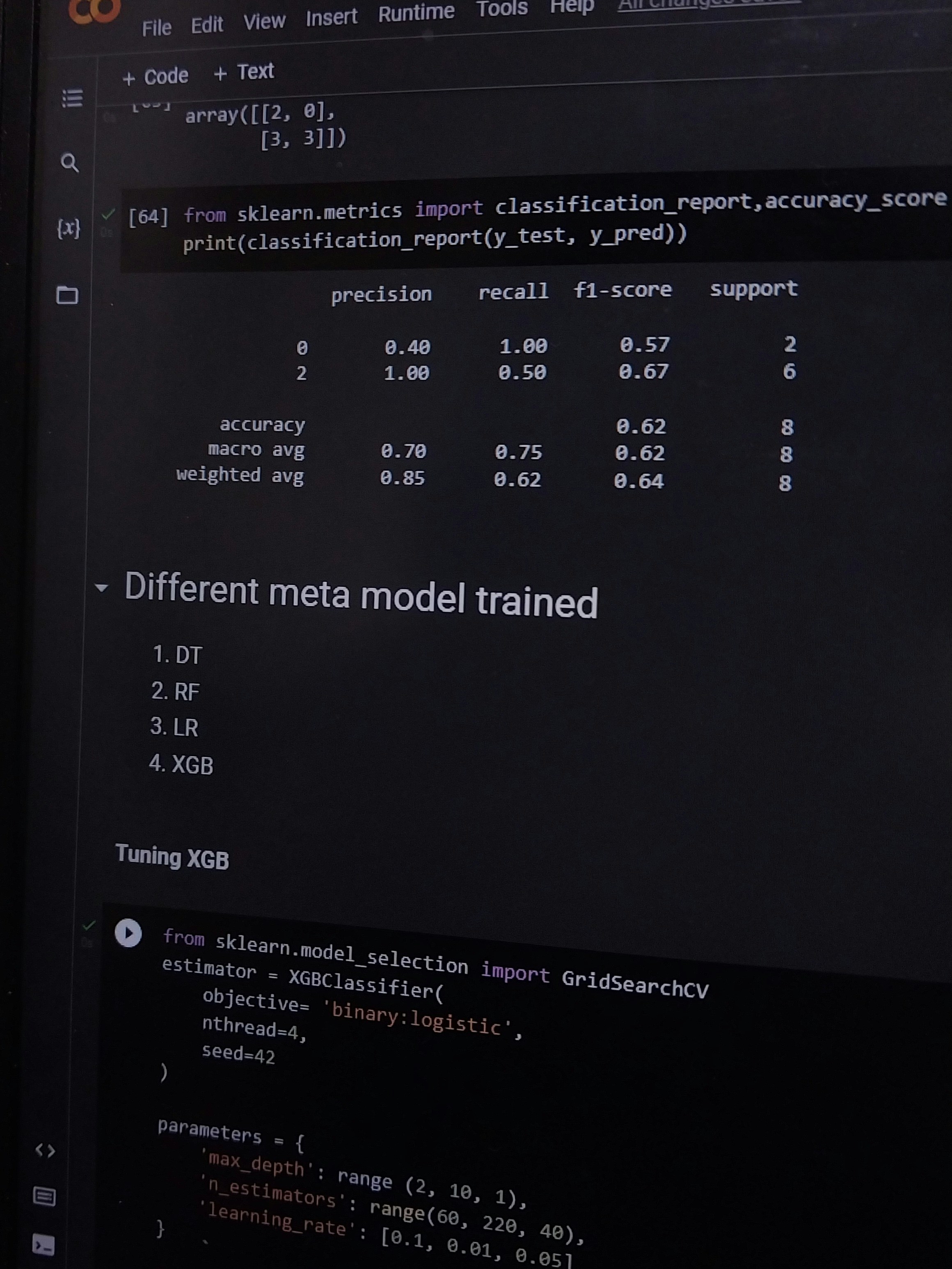
From these values, several key performance metrics can be derived. Accuracy, for instance, is determined by the formula: (TP + TN) / (TP + FP + TN + FN). This metric reflects the overall effectiveness of the model in classifying both positive and negative instances.
Precision, another vital metric, is calculated as TP / (TP + FP). This figure illustrates the proportion of true positive results among all positive predictions, helping to understand the model’s reliability when it asserts a positive classification. Similarly, Recall, computed as TP / (TP + FN), highlights the model’s ability to identify all actual positive cases, revealing its sensitivity.
Lastly, the F1 score offers a balanced measure between precision and recall, articulated as 2 * (Precision * Recall) / (Precision + Recall). It is particularly useful when evaluating models with uneven class distributions. By interpreting these metrics derived from the confusion matrix, one can gain a clear and detailed understanding of a model’s performance, guiding improvements and adjustments for better predictive outcomes.
Evaluation Metrics Derived from Confusion Matrix
The confusion matrix serves as a foundational tool in classification tasks, enabling the calculation of various evaluation metrics that assess model performance. Among the primary metrics derived from this matrix are precision, recall, F1 score, and accuracy, each providing unique insights into the effectiveness of a model.
Precision is defined as the ratio of true positive predictions to the total predicted positives. Mathematically, it is expressed as:
Precision = True Positives / (True Positives + False Positives)
This metric is crucial when the cost of false positives is significant, emphasizing the model’s ability to make accurate positive predictions.
Recall, also known as sensitivity, measures the ratio of true positives to the total actual positives. The formula for recall is:
Recall = True Positives / (True Positives + False Negatives)
This metric is particularly important in scenarios where missing a positive instance could lead to serious consequences, such as in medical diagnoses.
The F1 score combines precision and recall into a single metric, offering a harmonic mean that balances both dimensions. It is calculated as:
F1 Score = 2 * (Precision * Recall) / (Precision + Recall)
This metric is valuable in situations where there is an uneven class distribution, allowing for a more balanced view of model performance.
Lastly, accuracy is a straightforward metric that indicates the proportion of correctly classified instances out of the total instances. It is calculated as:
Accuracy = (True Positives + True Negatives) / Total Instances
While accuracy is easy to compute and understand, it can be misleading in imbalanced datasets where one class dominates the others.
Understanding these metrics derived from the confusion matrix is essential for effectively evaluating and fine-tuning models in various applications. They provide critical insights that facilitate informed decisions about model deployment and refinement.
Confusion Matrix in Practice: Real-World Examples
The confusion matrix serves as a fundamental tool in evaluating the performance of classification algorithms across various domains. In healthcare, for instance, it plays a crucial role in diagnosing diseases. When a medical imaging algorithm analyzes X-rays or MRIs, the confusion matrix can assess how accurately the algorithm identifies conditions, such as cancer. By categorizing predictions into true positives, false positives, true negatives, and false negatives, healthcare practitioners can gauge the effectiveness of the tool. Misclassifications can lead to serious consequences, emphasizing the matrix’s importance in improving diagnostic accuracy.
Another domain where the confusion matrix is vital is finance. Financial institutions often rely on predictive modeling to detect fraudulent transactions. By employing a confusion matrix to analyze the outcomes of fraud detection algorithms, banks can identify the frequency of successful detections versus missed cases. Such metrics enable financial analysts to refine their models, thereby enhancing security measures against fraud. For instance, if a bank’s model shows a high rate of false negatives, it might indicate a need for better training data or algorithm adjustments.
Moreover, image classification, a prominent area in artificial intelligence, also benefits significantly from confusion matrices. For example, when developing a model to classify images of animals, the confusion matrix helps quantify how many images of cats were mistakenly classified as dogs. By analyzing such data, developers can identify specific weaknesses in their model and make necessary improvements to ensure accurate classifications. This iterative process of evaluation and refinement underlines the crucial role of confusion matrices in enhancing model reliability in real-world applications.
Common Challenges and Limitations of Confusion Matrices
Confusion matrices, while valuable tools for understanding the performance of classification algorithms, come with a set of challenges and limitations that analysts need to be aware of to avoid misinterpretations. One significant issue is class imbalance. In scenarios where one class heavily outnumbers another, the confusion matrix may portray an optimistic view of model performance. For example, in a binary classification task where 95% of instances belong to class A and only 5% to class B, a model could achieve high accuracy by predominantly predicting class A. However, such an approach might overlook the poor performance on the minority class, leading to misleading conclusions about the model’s effectiveness.
Another challenge lies in the potential complexity of interpreting the results of a confusion matrix, especially in multi-class classification problems. With multiple classes, the matrix grows in size and can complicate the assessment of individual class performances. This can lead to difficulties in identifying which classes the model is struggling with, and adjustments may be needed to address such issues. It becomes crucial to investigate precision, recall, and F1-score, which help to provide a more nuanced view of performance across all classes.
To mitigate these challenges, practitioners should utilize techniques such as stratified sampling to ensure that training and testing datasets reflect the original class distribution, thereby reducing the effects of class imbalance. Additionally, employing metrics like area under the ROC curve (AUC-ROC) and utilizing k-fold cross-validation can help ensure that models are evaluated comprehensively. By maintaining a balanced perspective when interpreting confusion matrices and supplementing them with other evaluation metrics, analysts can enhance their understanding of model performance and make informed decisions based on the results.
Advanced Visualization Techniques for Confusion Matrices
Understanding the performance of machine learning models is crucial, and confusion matrices serve as a fundamental tool in this assessment. To enhance the interpretability of confusion matrices, advanced visualization techniques can be invaluable. One popular method is the use of heatmaps, which graphically represent the data contained in a confusion matrix, portraying both the volume of predictions and their accuracy in a visually appealing format.
Heatmaps convert numerical values into a color-coded system, allowing practitioners to quickly identify patterns, such as classes with higher misclassification rates or an imbalance in predictive accuracy across classes. Libraries like Matplotlib and Seaborn in Python provide robust functions to create heatmaps easily. For example, a basic heatmap can be generated using Seaborn’s heatmap() function, which offers various options for customizing the visuals, such as adding annotations and adjusting color scales.
Additionally, more advanced graphical representations include 3D visualizations and interactive dashboards. Using libraries such as Plotly and Bokeh, developers can create immersive representations of confusion matrices. These tools enable users to zoom in on specific sections of the matrix or observe changes over time, providing deeper insights into model performance and class interactions.
Furthermore, tools like TensorBoard and Yellowbrick provide comprehensive solutions for visualizing confusion matrices along with other model performance metrics. They facilitate the comparison of various models, helping in choosing the best one based on visual insights rather than relying solely on numerical scores.
In conclusion, incorporating advanced visualization techniques for confusion matrices not only enhances understanding but also contributes to better decision-making in model evaluation and selection. Embracing these visual tools can significantly improve the interpretability and usability of confusion matrices in machine learning applications.
Conclusion and Future Directions
The significance of confusion matrices in evaluating the performance of machine learning models cannot be overstated. This powerful tool provides a detailed insight into how well a model is making predictions, particularly in the context of classification tasks. By summarizing the true positive, false positive, true negative, and false negative rates, confusion matrices enable practitioners to assess not just the overall accuracy of a model but also its strengths and weaknesses in making specific classifications. Such comprehensive metrics make it easier to identify issues related to predictive performance, leading to targeted improvements.
As machine learning continues to evolve, the role of confusion matrices may also transform. A potential future direction involves the integration of confusion matrices with more advanced metrics and visualizations. As models become increasingly complex with deeper architectures or ensemble methods, combining traditional confusion matrix insights with techniques like ROC curves or precision-recall curves may provide a more nuanced understanding of model performance. This kind of multidimensional approach could help practitioners better interpret outcomes, especially in critical applications like healthcare or finance.
Moreover, advancements in interpretability and explainable AI may cause confusion matrices to be adapted for richer contexts, where model decisions need to be more transparent. This might include real-time monitoring solutions that update confusion matrices dynamically as new data become available, allowing for continuous evaluation and refinement of models in production settings.
In conclusion, as machine learning technologies and methodologies advance, confusion matrices will likely remain a fundamental tool for model evaluation, while also adapting to incorporate new insights and techniques for improved interpretability and usability. Keeping abreast of these trends will be crucial for practitioners aiming to harness the full potential of their models.