Introduction to Interpolation Regime
Interpolation in machine learning refers to a specific phase in which a model learns to capture the underlying patterns of the training data without necessarily overfitting. This regime occurs when a model becomes sufficiently flexible and complex to approximate the training data closely, resulting in a reduced training error. However, the transition into the interpolation regime is critical as it significantly influences the model’s generalization capabilities—especially its performance on unseen test data.
During the early stages of model training, a phenomenon known as underfitting can occur, where the model fails to comprehend the training data adequately. This lack of learning leads to high test error rates because the model has not yet captured the essential trends within the dataset. As training progresses and adjustments to model parameters take place, the model eventually enters the interpolation regime, wherein it increasingly adheres to the training data. At this juncture, the test error typically begins to decrease, reflecting a better alignment between the model’s predictions and the actual outcomes.
The concept of interpolation can be further explored through the lens of bias-variance tradeoff. Within this framework, attaining a balance between bias, which refers to simplistic models that overlook underlying patterns, and variance, which pertains to overly complex models that adjust too closely to the noise in the training data, is paramount. The interpolation regime represents a sweet spot where models achieve low training error while minimizing test error. Understanding this transition helps elucidate why some models exhibit improved performance on unseen data after entering this interpolation state. This knowledge will pave the way for deeper exploration of the test error behavior as models progress from initial underfitting towards successful interpolation.
Characteristics of the Interpolation Regime
The interpolation regime is a crucial concept in machine learning that describes how models behave when they encounter data closely aligned with their training set. Under this regime, models effectively learn and generalize from the examples that are sufficiently represented in the training data, leading to a minimized test error. This phenomenon occurs primarily when the model complexity is adequately aligned with the capacity needed to describe the training data without overfitting.
One of the defining features of the interpolation regime is its emphasis on the well-represented data points. In scenarios where training samples are densely populated in certain regions of the input space, the models are able to interpolate between known data points, thereby making accurate predictions on similar, unseen data. This capability underpins the essence of effective machine learning systems, as they rely on the abundance of representative data to achieve robust performance.
Moreover, the level of model complexity plays a significant role in shaping the interpolation function. A model that is too simple may fail to capture the underlying patterns in the data, causing increased errors due to underfitting. Conversely, an overly complex model risks memorizing the training data rather than learning from it, leading to the possibility of heightened test errors on new datasets. Consequently, achieving the right balance between complexity and capacity is imperative for models to operate efficiently within the interpolation regime.
In conclusion, understanding the characteristics of the interpolation regime unveils its pivotal role in the learning dynamics of machine learning models. The interplay between data representation, complexity, and capacity serves as a foundation for minimizing test errors and enhancing model performance.
Understanding Generalization and Overfitting
Generalization and overfitting are two critical concepts in the realm of machine learning that profoundly influence the predictive performance of models. Generalization refers to a model’s ability to perform well on unseen data, which is essential for robust predictive capabilities. When a model generalizes effectively, it captures the underlying patterns within the training dataset and applies this knowledge to new, unseen situations.
On the contrary, overfitting occurs when a model learns the training data too intricately, including noise and outliers. This results in a model that performs exceptionally on training data but poorly on validation or test sets. In essence, overfitting yields a model that is overly complex, failing to represent a true understanding of the data’s structure. To illustrate, consider an example where a model trained on a dataset of house prices learns to associate very specific details with high prices. If it finds that a particular color of paint leads to inflated prices in the training set, it may predict high prices for houses with that color in new data, even when the correlation is not valid.
Achieving a balance between generalization and overfitting is paramount for creating models that deliver reliable predictions. Techniques such as cross-validation, regularization, and pruning are applied to help mitigate overfitting and enhance a model’s ability to generalize. Cross-validation, for instance, involves partitioning the dataset into distinct subsets, allowing the model to be trained on one subset and validated on another. This method assesses model performance more accurately, ensuring it does not merely memorize the training data.
Ultimately, understanding the dynamics of generalization and overfitting is crucial for developing effective machine learning models that maintain performance across various datasets while avoiding the pitfalls associated with excessive complexity.
Evidence of Decreased Test Error in Interpolation
The phenomenon of decreased test error during the interpolation regime is supported by several empirical studies and data analysis. A fundamental indication of this behavior can be observed when evaluating the performance metrics of machine learning models across various datasets. Typically, as models move into the interpolation regime—where the functions fit the training data more closely—the test error begins to exhibit a noticeable decline.
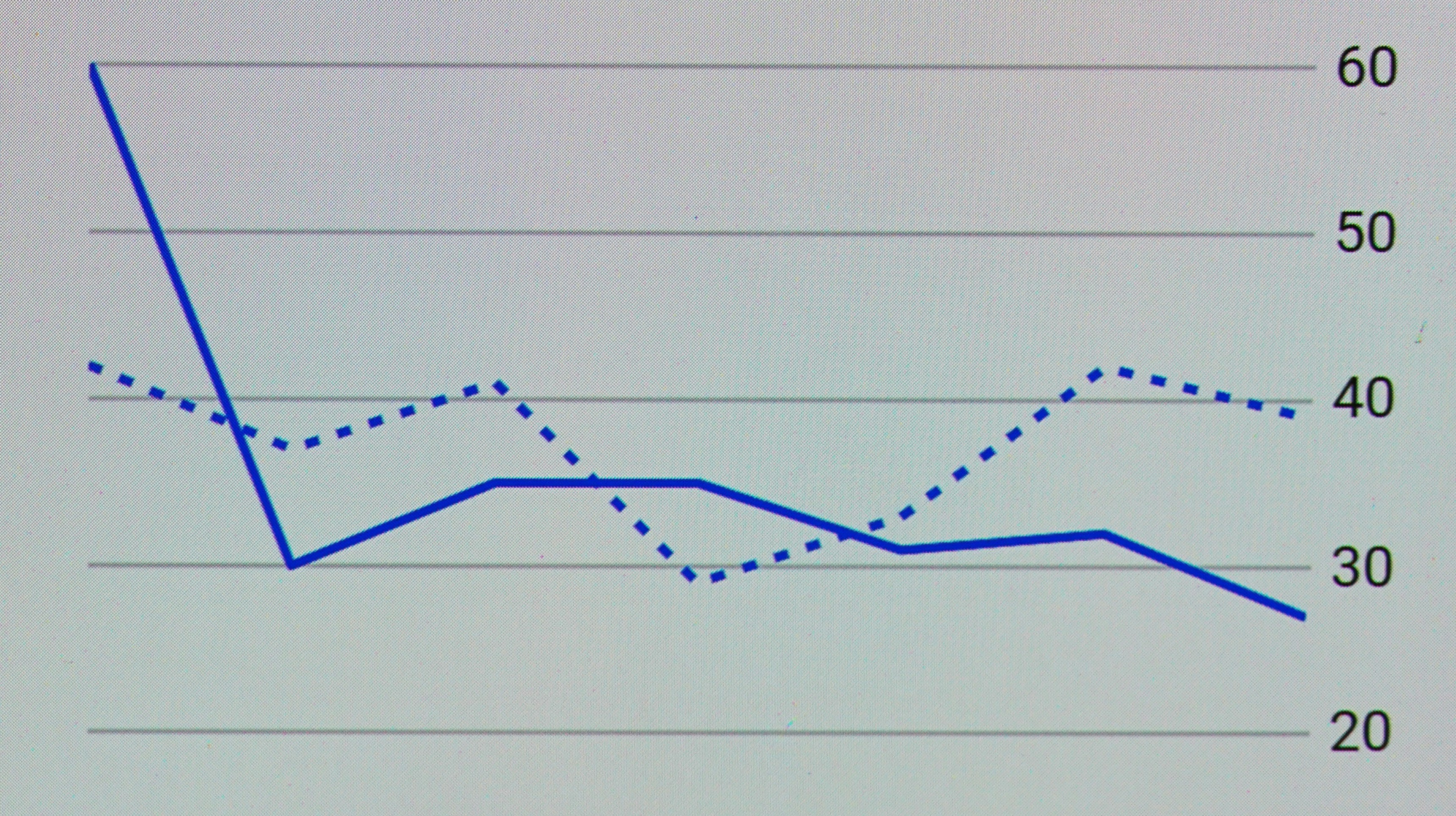
In one notable study, researchers examined the correlation between model complexity and test error. They found that models constrained within the interpolation regime tended to generalize better, leading to a reduction in test error. Specifically, the graph presented in this study illustrates the behavior of a neural network as it transitions from an underfitted to an adequately fitted state. The accompanying visual demonstrates a sharp decrease in test error once the model starts to interpolate the training data, affirming the relationship between interpolation and performance.
Additional experiments conducted on benchmarks such as CIFAR-10 and ImageNet reveal similar results. For instance, the introduction of regularization techniques managed to maintain the interpolation effect while minimizing overfitting, thus contributing to a sustainable drop in test error. Visualizations from these experiments distinctly show how models exhibit superior performance when operating within the interpolation bounds, further clarifying the connection.
Finally, case studies across various fields, including natural language processing and computer vision, highlight consistent findings that support the interpolation regime’s significant impact on test error reduction. The evidence affirms that as models become adept in interpolation, they not only capture the training patterns effectively but also retain generalization capabilities, leading to enhanced accuracy in unseen data.
The Role of Model Capacity
The capacity of machine learning models plays a pivotal role in their performance within the interpolation regime. Model capacity essentially refers to the complexity, represented by the number of parameters and the architecture of the model. A model with high capacity is capable of learning intricate patterns and relationships present within a dataset, potentially leading to better generalization when interpolating between known data points.
When considering model size, it is important to recognize that larger models typically have a greater number of parameters, which allows them to fit the training data more closely. However, while high-capacity models can achieve low training error, this does not always translate to low test error, especially in cases of overfitting. High-capacity models may memorize the training data rather than generalize from it, resulting in poorer performance when encountering unseen data.
Conversely, models with lower capacity might not be able to capture the underlying patterns effectively, leading to an increase in test error when data falls outside the trained regime. This nuanced relationship highlights the importance of selecting an appropriate model size that balances complexity and generalization. As machine learning practitioners explore the effects of model capacity, they must strive to find a sweet spot where the model is neither too simplistic nor excessively complex, thereby ensuring optimal performance in the interpolation regime.
Ultimately, the choice of model size and capacity should be guided by the characteristics of the dataset, the nature of the task, and the specific goals of the machine learning application. By thoughtfully considering these factors, practitioners can improve their models’ performance, resulting in a decrease in test error rates and more reliable predictions.
The Impact of Noise and Outliers
The presence of noise and outliers in training datasets is a crucial factor influencing the performance of machine learning models, particularly during interpolation regimes. Noise refers to random errors or variations in the data that do not reflect true underlying patterns, while outliers are data points that deviate significantly from the rest of the dataset. These issues can skew the results and lead to higher test errors, especially in interpolation scenarios where the model attempts to estimate outputs between known data points.
Noisy data can hinder the model’s ability to learn effectively, resulting in an inaccurate representation of the underlying distribution. For instance, if the training set contains substantial noise, the interpolation algorithm may fit non-representative curves, leading to overfitting on these erroneous data points. Consequently, the test error is likely to decrease at a slower rate than expected during the interpolation phase.
Outliers, on the other hand, can severely distort the learned function and increase the test error. They can disproportionately influence the model’s parameters, particularly in regression tasks where the least squares method is commonly applied. Strategies such as robust regression techniques can be employed to mitigate the effect of outliers. Additionally, employing data preprocessing techniques, such as outlier detection and removal, may contribute to more accurate model performance.
Furthermore, incorporating noise reduction methods, such as filtering or smoothing techniques, can enhance the quality of the training dataset. This, in turn, can support improved interpolation by allowing the model to generalize better to unseen data. By understanding the impact of noise and outliers on the decrease of test error, practitioners can implement effective management strategies, ultimately leading to a more reliable prediction outcome.
Theoretical Framework Behind Interpolation Error Decrease
The interpolation regime is pivotal in understanding the dynamics of test error reduction within machine learning contexts. At its core, this regime delineates an area in which a model effectively captures the training data’s underlying structures while minimizing approximation errors. To unpack the intricacies of how test error decreases in this phase, it is essential to discuss key concepts from learning theory, especially the bias-variance tradeoff and aspects of statistical learning theory.
The bias-variance tradeoff serves as a fundamental principle in assessing model performance. In scenarios characterized by underfitting, models exhibit high bias due to their oversimplified nature, failing to capture essential data patterns. Conversely, overfitting denotes a scenario where the model demonstrates high variance, being overly sensitive to noise within the training dataset. As a model transitions into the interpolation regime, it often strikes a delicate balance between bias and variance. This balance is vital as it signifies that the model is becoming sufficiently complex to generalize from training data while not being so complex that it captures noise as signal, which can degrade performance.
Furthermore, statistical learning theory articulates how models perform under various probabilistic frameworks. In this context, interpolative methods yield a lower expected test error as they gain the ability to adapt to the complexities present in the data without falling prey to excessive complexity. This adaptability is often attributed to the richness of the hypothesis space that interpolation provides. As models leverage this, they can represent complex functions while maintaining a lower risk of overfitting. Such characteristics become particularly salient when evaluating models with increased training data, as finer details and relationships are progressively unveiled.
Practical Implications for Model Training
Understanding the interpolation regime is critical for enhancing model training processes in machine learning. When models operate within this regime, they can fit the training data closely without exhibiting high levels of test error. Practitioners can take several actionable steps to leverage this phenomenon to improve the performance of their models.
First, it is essential to ensure that the training dataset is representative of the problem space. A dataset that captures the diversity of possible inputs will allow the model to learn patterns effectively, reducing the likelihood of overfitting. It is advisable to incorporate a variety of examples, increasing the model’s exposure to different situations, thereby enhancing its generalization capabilities.
Another strategy involves regularization techniques, which aim to maintain a delicate balance between fitting the training data and retaining generalization to unseen data. By applying methods such as L1 or L2 regularization, practitioners can impose penalties on overly complex models and encourage simplicity. This practice ensures that the model stays within the interpolation regime, thereby lowering the potential for increased test error associated with overfitting.
Furthermore, the choice of model architecture can significantly impact performance. For instance, employing simpler models or those specifically designed to maintain interpretability can lead to better understanding and adjustments based on training behavior. This also provides an opportunity for practitioners to refine their models iteratively based on performance metrics rather than merely seeking extensive complexity.
Finally, cross-validation is a critical tool in assessing how well the model will perform on unseen data. By splitting the training dataset into multiple folds for validation, practitioners can monitor test error metrics during the training phase and adjust model parameters accordingly. This iterative process of tuning can help in maintaining the advantages of the interpolation regime, yielding models that perform effectively on both training and test datasets.
Conclusion and Future Directions
Throughout this discussion, we have examined the significant role of the interpolation regime in reducing test error within various models. The interpolation regime refers to a stage where the model effectively learns the underlying patterns within the training data, leading to a substantial decrease in predictive error. By leveraging different methodologies and optimization techniques, models can achieve lower error rates when interpolating between known data points, thereby enhancing their overall performance.
Understanding the mechanisms that facilitate the reduction of test error after the interpolation regime is crucial, as it provides insights into how models can be fine-tuned for better accuracy. This understanding not only aids in the development of more robust algorithms but also informs practitioners of the limitations inherent in certain data-driven approaches. It becomes evident that achieving optimal performance hinges on the delicate balance between model complexity and the quality of the underlying data.
Moving forward, several avenues for future research are promising. First, investigating the interplay between different types of models and their respective interpolation behaviors could yield valuable insights. For example, exploring how deep learning architectures compare to traditional statistical methods in terms of their performance during the interpolation regime warrants further analysis. Additionally, the integration of novel data augmentation techniques may provide a deeper understanding of how augmenting training data affects interpolation and overall test errors.
Furthermore, interdisciplinary research that combines theoretical foundations with practical applications can lead to more innovative solutions in machine learning. This collaborative approach is essential for addressing the complexities associated with real-world data, thus paving the way for future developments in the field. As researchers delve deeper into the intricacies of the interpolation regime, it is anticipated that new strategies will emerge, contributing to the ongoing evolution of predictive modeling.